AI Scaling Laws: Kaplan vs. Chinchilla and Why Training Recipes Matter

Quick answer: AI scaling laws estimate how model size, training data, and compute trade off under a fixed budget. Kaplan and Chinchilla reached different recipes because experimental choices matter: a curve that looks clean can still reflect an undertrained model or a learning-rate schedule rather than a universal law.

In the previous piece, built around Lilian Weng's "Scaling Laws, Carefully", we looked at one of the most important mathematical ideas behind generative AI:

Model capability, parameter count, training data, and compute often follow predictable power-law relationships.

This article is the sequel.

Diogo Almeida's "Scaling Laws, Honestly" adds an important reality check. Scaling laws matter, but they are not magic. They do not say, "make the model bigger and the result will automatically improve." Their real value is more practical:

Should the next dollar go into a larger model or more training data?
Can small experiments predict a much larger training run?
Does a clean line on a log-log chart reflect a real law, or a hidden training setting?
For companies and investors, which AI stories are just parameter-count worship, and which show a repeatable return curve?

Here is the blunt version:

Diogo is not rejecting scaling laws. He is warning that weak experimental design can dress up a bad training recipe as a mathematical law.

That matters commercially. In AI, the dangerous mistake is not only misunderstanding math. It is treating an uncalibrated dashboard as if it were a steering wheel.

The 16-Year-Old Version

Imagine you are training a student for a very hard exam.

You can spend money on three things:

Give the student a bigger brain. That is like increasing model parameters $N$ .
Give the student more practice problems. That is like increasing training tokens $D$ .
Give the student more study time and better teachers. That is like increasing total compute $C$ .

At the end, you do not care how big the student's brain is. You care about the error rate on the exam. In model training, that error score is called loss $L$ .

The early Kaplan-style intuition was roughly:

When the budget grows, make the brain bigger first. The number of exercises does not need to grow as quickly.

The Chinchilla correction was:

Many students are not limited by brain size. They are undertrained. Brain size and exercise volume need to grow together.

Diogo adds another sentence:

If the big-brain students all receive roughly the same amount of practice, and the learning speed is gradually reduced to zero near the end, the experiment may make extra practice look less useful than it really is.

That is the story.

The formulas below are all trying to answer one simple question:

With the same training budget, should we buy a bigger brain or more practice?

The Four Variables

For language-model training, keep four quantities in your head:

$N$ : number of parameters. Think brain capacity or factory size.
$D$ : training tokens. Think practice problems or raw material.
$C$ : training compute. Think total study budget, electricity, and machine time.
$L$ : loss. Think exam error rate; lower is better.

Training compute is often approximated as:

C \approx 6ND

The meaning is simple: a bigger factory processing more raw material needs more electricity and machine time.

A simplified scaling-law formula writes loss as:

L(N, D) = E + \frac{A}{N^\alpha} + \frac{B}{D^\beta}

Do not let the symbols intimidate you. The formula says three plain things:

$E$ is the noise floor that is hard to remove.
Increasing model size $N$ lowers loss, but with diminishing returns.
Increasing data $D$ also lowers loss, again with diminishing returns.

So the business question becomes:

Under a fixed budget, should we buy more model capacity or more training data?

That is the heart of the Kaplan versus Chinchilla disagreement.

Kaplan vs. Chinchilla

OpenAI's 2020 Kaplan scaling laws leaned toward larger models. As compute increased, the compute-optimal model size should grow faster than the training-data volume.

DeepMind's 2022 Chinchilla paper argued that many large models were too big and undertrained. Under a fixed compute budget, the better recipe was often a smaller model trained on more tokens.

The difference is easiest to see as a table:

Question	Kaplan-style answer	Chinchilla-style answer
When compute grows, what grows first?	Mostly parameters $N$	Parameters $N$ and data $D$ grow together
What does the optimal model look like?	Larger, not necessarily trained as fully	Smaller, but trained more fully
Representative exponent	$N_{\text{opt}} \propto C^{0.73}$	$N_{\text{opt}} \propto C^{0.50}$
Business translation	Buy more capacity	Match capacity with raw material

If training compute rises 10x, the two recipes look different:

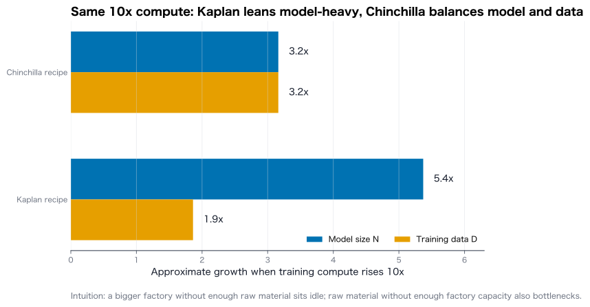
Kaplan versus Chinchilla resource allocation under 10x compute

Figure 1: With the same 10x increase in compute, the Kaplan-style recipe expands the model more aggressively, while Chinchilla keeps model and data growth closer together.

This is not a tiny academic disagreement. It can change hundreds of millions of dollars in training budgets.

For enterprise buyers, it changes whether you worship "the largest model" or ask whether a model is trained well enough for your task at a usable cost.

For investors, it changes whether you look only at GPU cluster size or also ask about data quality, training recipes, inference cost, and product feedback loops.

The next two Python figures turn the formula into geometry. The first is a 2D contour map: the horizontal axis is model size, the vertical axis is training data, and the white diagonal lines are fixed-compute budgets. The second is a 3D surface: loss behaves like a valley, and training strategy is the act of finding the lowest point allowed by the budget.

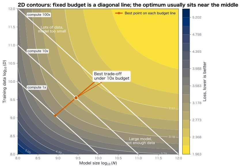
Scaling law loss contour with fixed compute lines

Figure 2: Brighter regions mean lower loss. A fixed budget is a diagonal line. The best point is not simply far right or far up; it is the balance between model and data.

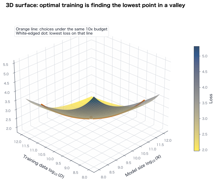
Scaling law loss surface with compute-optimal valley

Figure 3: In 3D, compute-optimal training looks like moving along a budget line and finding the lowest point in the valley.

An animation makes the point even clearer. As budget moves from 1x to 100x, the white budget line moves outward. The red point is the best trade-off under each budget.

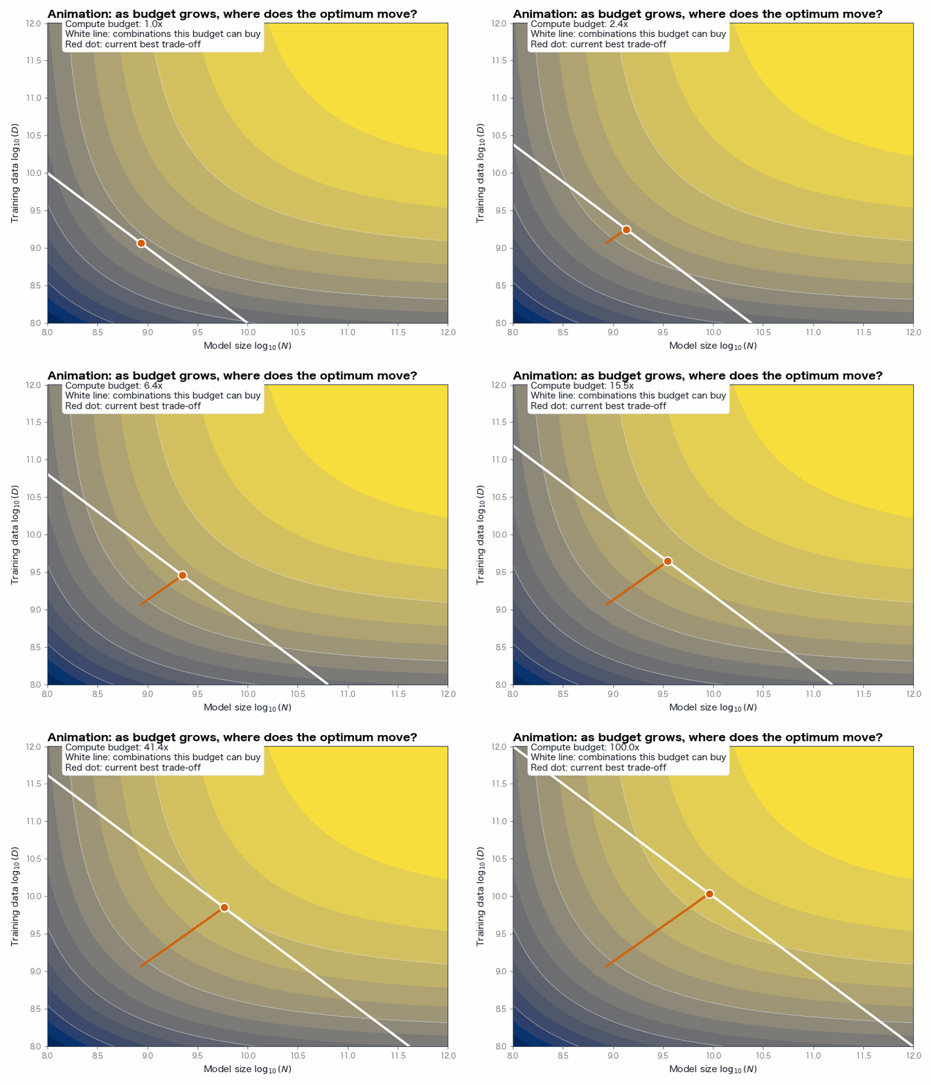
Animated scaling law budget frontier

Figure 4: More budget does not mean "move right forever." The optimal path usually grows model and data together.

You can also play with the sandbox below. It is not trying to be a research-grade simulator. It is for intuition: when model returns or data returns change, watch where the gold point moves.

Interactive Scaling Law Explorer

Drag the sliders to see where the budget should go

Think of the model as the factory and training data as the raw material. Darker color means lower loss; the gold point is the best trade-off for the current budget.

Value of a larger model0.34Higher means expanding the factory reduces mistakes more effectively.Value of more data0.36Higher means adding exercises and raw material reduces mistakes more effectively.Compute budget multiplier10xWith a fixed total budget, money spent on a larger model leaves less budget for training material, and vice versa.

Current compute-optimal growth rule

Model size: N_opt ∝ C^0.51

Training data: D_opt ∝ C^0.49

When both exponents are close to 0.5, it behaves like Chinchilla: factory and raw material grow together.

2D: loss map

Gold line is the fixed-compute constraint

3D view: loss surface

Lower means fewer mistakes

With the same 10x compute increase, how do the recipes spend it?

Kaplan-style

Parameters N5.4x

Data D1.9x

Chinchilla-style

Parameters N3.2x

Data D3.2x

When you use it, remember three things:

The horizontal axis is model size.
The vertical axis is training data.
The gold point is the best trade-off under the current compute budget.

What Is the Bug Diogo Points To?

Diogo calls the issue in the Kaplan setup a bug. I would translate it this way:

A hidden factor entered the experiment, making it look as if larger models mattered more than more data.

The paper wanted to estimate:

L = f(N, D)

meaning loss as a function of parameters and data.

But real training also contains hidden settings $S$ :

L_{\text{true}} = f(N, D, S)

$S$ includes learning-rate schedules, number of training steps, data repetition, tokenizer details, optimizer choices, and other training settings.

If $S$ is not controlled well, you may think you are measuring "what happens when the model gets bigger", while you are also measuring "whether the training recipe pressed the brake too early."

It is like trying to study the relationship between car horsepower and speed, while forgetting that different cars have different amounts of brake pressure applied. The curve may look smooth, but it is not measuring horsepower alone.

Step 1: Fixed Tokens Can Leave Big Models Undertrained

In much of the Kaplan setup, different model sizes were trained with a fixed token count. Diogo argues that this can create a problem: a small model and a large model may see the same number of tokens, but each parameter in the large model receives much less training signal.

Simplify it like this:

Model parameters $N$	Training tokens $D$	Tokens per parameter $D/N$
1B	130B	130
10B	130B	13
100B	130B	1.3

The business intuition is strong:

The larger the factory, the more raw material it needs. Otherwise the extra capacity sits underused.

If big models are not fed enough data, extra data can appear less important than it really is. The problem is not that data has no value; it is that the experimental setup did not explore the data axis fully enough.

In linear algebra language, parameters create a huge space of degrees of freedom. More degrees of freedom require more observations to constrain them.

In student language: a bigger brain can learn more, but it still needs enough practice problems to turn capacity into skill.

Step 2: Learning Rate Decay Can Make Training Look Saturated

Parameter updates can be written roughly as:

\theta_{t+1} = \theta_t - \eta_t \nabla L(\theta_t)

Here:

$\theta_t$ is the model's parameters at step $t$ .
$\nabla L(\theta_t)$ tells the model which direction reduces error.
$\eta_t$ is the learning rate, or how large each step is.

Kaplan used a schedule that warms up and then decays toward zero. A simplified cosine decay is:

\eta_t = \frac{\eta_0}{2}\left(1 + \cos\frac{\pi t}{T}\right)

As $t$ approaches the final training step $T$ , $\eta_t$ approaches zero.

The practical meaning:

When the learning rate is near zero, the model barely moves even if the gradient is still pointing toward improvement.

So the training curve can flatten and look "done." Diogo's reminder is that this may not prove more data stopped helping. It may only mean the schedule slowed learning almost to a stop.

Cosine learning rate decay to zero

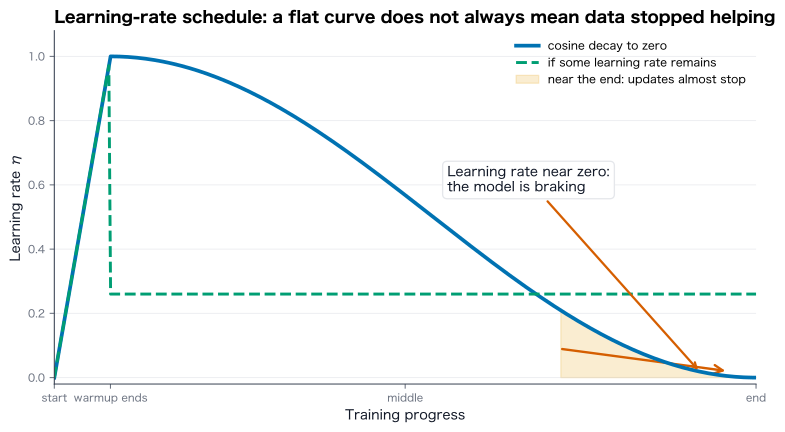
Figure 5: If the learning rate decays toward zero near the end, a flat loss curve may mean the model is barely updating, not that data has no value.

The animation looks like braking:

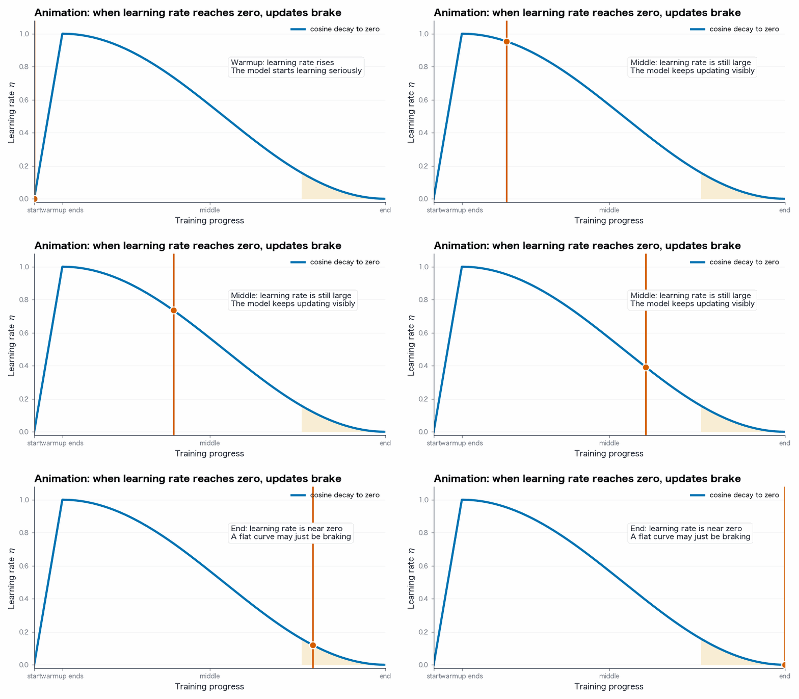
Animated learning rate decay progress

Figure 6: Near the end of training, the learning rate becomes tiny. The model may still have a gradient, but the update step is almost frozen.

Combine fixed token counts with a learning rate that goes to zero, and it becomes harder to see that larger models may still need more data.

Step 3: A Local Result Was Treated Too Generally

Diogo's third point is subtle.

If you only look inside a world where maximum token count is fixed and the learning-rate schedule decays to a particular endpoint, it may be true that the result looks insensitive to schedule inside that small world.

But scaling laws are used for a larger question:

When compute, parameters, and data all keep growing, how should we allocate them?

That is extrapolation.

In plain language: you watched a few quizzes and used them to predict the final exam. The line may look beautiful, but a small slope error can become a huge budget error.

loss L
^
|\
| \     small experiment region: looks straight
|  \
|   \____
|        \        extrapolation region: a tiny slope error
|         \____   becomes a huge budget error
+--------------------------> scale log(N), log(D), log(C)

This is also why Lilian Weng repeatedly emphasizes careful measurement: scaling-law forms can be clean, but their fits are sensitive to definitions, experimental range, loss precision, and training setup.

The Mathematical Essence: Scaling Laws Compare Marginal Returns

Return to the central formula:

L(N, D) = E + \frac{A}{N^\alpha} + \frac{B}{D^\beta}

Compute is fixed:

C \approx 6ND

So if $C$ is fixed, data can be written as:

D = \frac{C}{6N}

Substitute that into the loss function:

L(N) = E + A N^{-\alpha} + B\left(\frac{C}{6}\right)^{-\beta}N^\beta

This equation is worth reading slowly.

The first term, $A N^{-\alpha}$ , says a larger model lowers loss.

The second term, $B\left(\frac{C}{6}\right)^{-\beta}N^\beta$ , says that under a fixed compute budget, a larger model leaves less budget for data, which increases loss.

So the optimum is not "bigger is always better." It is where the two forces balance.

If you take the derivative with respect to $N$ and set it to zero, you get:

\alpha A N^{-\alpha-1} = \beta B\left(\frac{C}{6}\right)^{-\beta}N^{\beta-1}

You do not need to memorize the derivation. The business translation is:

The optimal training scale is where the last dollar spent on more model capacity and the last dollar spent on more data reduce loss by about the same amount.

That is the essence of scaling laws. They are not worshipping scale. They are comparing marginal return.

So if an experimental setup makes the marginal value of data look too low, the conclusion will lean toward larger models. If the experiment scans model size and token budget more systematically, the conclusion moves back toward balanced growth.

What This Means for Companies

First, do not buy models by parameter count.

Parameter count is capacity, not business value. Companies really buy:

error rate on the target task,
cost per call,
latency,
controllability and compliance,
integration into the workflow.

A 70B model that is well trained, cheap to serve, and stable on your evaluation set may be more useful than a 175B model that is expensive, slow, and hard to govern.

Second, data governance is not IT housekeeping. It is part of the AI balance sheet.

If the Chinchilla direction is right, data is not a minor input. It is a capital asset that must grow with model capacity. Companies should ask:

Which business data is high quality, low duplication, and legally usable?
Which expert feedback can be captured continuously?
Which errors have clear business cost and can become evaluation sets?
Which workflows let the model learn more about the business as it is used?

Third, the training curve must connect to the business curve.

Lower pretraining loss does not automatically mean higher ROI.

Companies need their own mapping:

\Delta L \rightarrow \Delta \text{business error rate} \rightarrow \Delta \text{cash flow}

For example:

Customer support: does a lower error rate reduce human escalation?
Finance: does better extraction reduce review time?
Sales: does better generation improve reply rate?
Legal: does lower hallucination reduce compliance risk?

If that mapping does not exist, a stronger model is still just a demo.

What This Means for Investment Judgment

This is not investment advice. It is a framework for analyzing AI companies and the AI supply chain.

I would split AI investment judgment into three curves:

Curve	Question to ask	Good signal	Danger signal
Technical curve	Do small experiments predict large training runs?	Stable scaling curves and real extrapolation checks	Only talking about parameter count, leaderboards, and announcements
Cost curve	Is the cost per unit of capability falling?	Inference cost, latency, and throughput improve	Revenue growth depends on rising COGS
Data curve	Does data become more valuable with use?	Proprietary data, feedback loops, evaluation sets	Generic, duplicated, or legally fragile data

If a company says, "we will win because we keep scaling", I would ask five questions:

Are you fitting training loss or real business metrics?
Has your small-scale extrapolation been verified by actual large training runs?
Are the tokens unique, high quality, and legally usable?
Does the revenue gained from a stronger model exceed the training and inference cost?
Can user feedback feed the next model or product advantage?

These questions sound simple. That is why they are useful. They filter out a lot of beautiful storytelling.

Reframing Several Industry Bets

First, GPUs and advanced packaging still matter, but the story becomes layered.

Chinchilla does not make compute unimportant. If model and data grow together, total training compute still rises. But the budget no longer serves only larger parameter counts. It also serves more high-quality tokens, longer training, and more sophisticated data pipelines.

Inference also becomes more important. Enterprises will not use one strongest model for everything. They will route tasks: cheap models for simple work, stronger models and more test-time compute for high-value work.

Second, data companies and vertical applications become more valuable.

If public internet text has declining marginal value, the scarce assets are:

industry-specific data,
expert annotation and review,
user behavior feedback,
high-quality evaluation sets,
products that route model outputs back into workflows.

These assets are harder to see on a financial statement than GPUs, but they may decide long-term gross margin and retention.

Third, open-source models will keep lowering the price of raw model capability.

As training recipes become clearer and the best model is not always the biggest one, many capabilities become cheaper and more commoditized. Business value moves from "we have a model" to:

we know which model to use when,
we have better data and evaluation,
we embed the model into real workflows,
we deliver the same result at lower cost.

That is crucial for investment judgment. The model itself may become infrastructure, while workflow, data loops, and distribution can still compound.

One-Sentence Summary

The previous article said:

Scaling laws turn AI training from blind spending into a large bet with instruments.

This article adds:

The instruments themselves must be calibrated. Otherwise the curve you see may be the shadow of the experimental setup.

The value of Diogo Almeida's "Scaling Laws, Honestly" is not drama about whether an old paper was wrong. Its value is the discipline it adds to reading AI curves:

What is the curve actually measuring?
Which variables are hidden?
Can the conclusion be extrapolated?
Can the technical metric become business cash flow?

For companies: do not buy the largest model. Buy the capability that best matches your error cost.

For investors: do not only ask who is scaling. Ask who can honestly measure the marginal return to scaling.

The next piece can continue from here: as training-time scaling gets more expensive, why test-time compute, agent workflows, model routing, and evaluation systems become the next commercial battlefield.

References

Diogo Almeida, Scaling Laws, Honestly, 2026.
Lilian Weng, Scaling Laws, Carefully, 2026.
Jared Kaplan et al., Scaling Laws for Neural Language Models, 2020.
Jordan Hoffmann et al., Training Compute-Optimal Large Language Models, 2022.
Tim Pearce and Jinyeop Song, Reconciling Kaplan and Chinchilla Scaling Laws, 2024.